In June 2026 I tried to determine the frequency of late printing variations within the first series of 1949 Leaf baseball cards. The initial reading of the data revealed a few cards whose implied frequency distributions were not compatible with a single traditional bell curve. This implied something else at play, which I hypothesized might be the presence of multiple distributions, such as what would be created if Leaf were to have adjusted cards in batches rather than at a single discrete point in the production cycle.
A mixture model was employed to determine if more than one batch existed, and if so, identify the component distributions and their relative weights. In short, how many times did Leaf stop the presses to “fix” their designs and how many cards were affected with each stoppage?
Mixture models can get hairy pretty fast for the typical Excel setup. I turned to R to work out the math and am including my code so others may learn from it and conduct their own research.
Data Prep:
R doesn’t need a lot of fluff. It will conduct its own transformations and needs only the most basic data with which to work. For my purposes, I created a .csv file consisting of three columns. As always when working with data like this, each row represents exactly one card, no spaces appear in column headers, there are zero merged cells, no formatting, and no summary or total rows.
| .CSV Column Heading | Description |
|---|---|
| card_name | Player name depicted on card |
| version_b | Number of observed examples of a late printing variation for that specific card |
| n | Number of TOTAL observations of that specific card |
My file can be found here.
R Programming
Step 1: Install Packages
R uses packages that greatly simply the process of setting up calculations and transforming data. For the purposes of this project, I used flexmix for the mixture model math and ggplot2 to be able to visualize the results with a forest plot. Installation of packages is a one-time deal. As a result, future projects can skip this step because their installation is persistent across future uses of the program.
install.packages("flexmix")   # mixture model engine
install.packages("ggplot2")   # visualisation
Step 2: Load Packages
Activate the recently installed flexmix and ggplot2 packages.
library(flexmix)
library(ggplot2)
Step 3: Import Data
Import the .csv file containing the sampled ’49 Leaf baseball card data. Make sure the “/” characters in your file path are leaning the correct way (my PC tends to flip these around the other way when I copy a file path). R is really fickle about this.
df <- read.csv("C:/Users/........./CardBoredom/49_Leaf_Study.csv", stringsAsFactors = FALSE)Step 4: Verify Data Loaded Correctly
Always good practice to make sure there isn’t some random comma throwing things out of line in the file.
head(df)      # shows first 6 rows
str(df)       # shows column types
nrow(df)      # should be 28
Step 5: Fit Models
My guess was that Leaf made changes to the printing plates at 2 or 3 different points in the production cycle. I tested for four different fits, 1 (in case there was a single event producing all the variations), 2-3 (my best guesses), and 4 (in case there were more than initially thought). Specifically, I applied an expectation-maximization (EM) mixture model to the data. It results in scoring various parameters, rewarding those that improve model fit and penalizing extraneous additions to the model.
set.seed(42)  # makes results reproducible

fit1 <- stepFlexmix(cbind(version_b, n - version_b) ~ 1,
                    data  = df,
                    k     = 1,
                    model = FLXMRglm(family = "binomial"),
                    nrep  = 20)

fit2 <- stepFlexmix(cbind(version_b, n - version_b) ~ 1,
                    data  = df,
                    k     = 2,
                    model = FLXMRglm(family = "binomial"),
                    nrep  = 20)

fit3 <- stepFlexmix(cbind(version_b, n - version_b) ~ 1,
                    data  = df,
                    k     = 3,
                    model = FLXMRglm(family = "binomial"),
                    nrep  = 20)

fit4 <- stepFlexmix(cbind(version_b, n - version_b) ~ 1,
                    data  = df,
                    k     = 4,
                    model = FLXMRglm(family = "binomial"),
                    nrep  = 20)
Step 6: Compare BIC and AIC
Here is where we start getting answers.
bic_table <- data.frame(
  k   = 1:4,
  BIC = c(BIC(fit1), BIC(fit2), BIC(fit3), BIC(fit4)),
  AIC = c(AIC(fit1), AIC(fit2), AIC(fit3), AIC(fit4))
)

print(bic_table)
This command produces a table with three columns. Each of the four models gets its own row in the table, along with the result of the BIC and AIC calculations. The model that best explains the data will have the lowest BIC. In the case of my data, fit2 held the most explanatory power, implying there were two distributions hiding inside the cards I had studied.
| MODEL | BIC (lower=better) | ΔBIC vs k=2 | AIC (lower=better) | ΔAIC vs k=2 | logL |
|---|---|---|---|---|---|
| fit1 (All Cards Changed at Once) | 185.9792 | +3.20 | 184.6470 | +5.87 | -91.32 |
| fit2 (Two Batches) | 182.7810 | — | 178.7844 | — | -86.39 |
| fit3 (Three Batches) | 189.4454 | +6.67 | 182.7844 | +4.00 | -86.39 |
| fit4 (Four Batches) | 196.1098 | +13.33 | 186.7844 | +8.00 | -86.39 |
A 2-6 point difference in BIC of between adjacent models is positive evidence of there being 2 distributions, but not overwhelming on its own. The 5.87 difference observed in AIC is much more meaningful, and in these results we see both measures in alignment that fit2 is the proper choice. Moving up to 3 or 4 batches adds zero additional fit to the model (logL is completely unchanged beyond fit2).
Step 7: Get the True Proportion for Each Group
flexmix fits a binomial GLM internally, so parameters come out on the log-odds scale. You need to back-transform them to proportions using the inverse logit.
log_odds <- parameters(fit2)

# Convert log-odds to probability
group_proportions <- exp(log_odds) / (1 + exp(log_odds))
print(group_proportions)
Step 8: Get the Mixing Weights
These are the proportions of cards belonging to each group, represented as a percentage of the 28 cards studied.
mixing_weights <- prior(fit2)
print(mixing_weights)
My results:
| Group 1 | Group 2 | |
|---|---|---|
| R Output | 0.8209132 | 0.2442725 |
| Implied number of Cards | 23 | 5 |
Step 9: Assign Cards to Most Likely Group
This will present a table containing a separate row for each card in the source file. The final column (“group”) will identify which of the two distributions each name appears to fall within. All cards will be assigned a group, regardless of how confident one may be in any particular assignment.
# Posterior probability of belonging to each group
post_probs <- posterior(fit2)

# Assign to the group with the highest posterior probability
df$group <- apply(post_probs, 1, which.max)

# Add the observed proportion for reference
df$prop_b <- df$version_b / df$n

# View the assignments
df[order(df$prop_b), c("card_name", "version_b", "n", "prop_b", "group")]
Step 10: Flag Ambiguous Groupings
Some cards might be borderline cases where a decent case can be made for grouping them into one distribution or the other. In this case, two cards sit right on the border between Group 1 and Group 2. The addition of a few more cards into the sample data might swing them more firmly in one direction or the other.
df$max_posterior <- apply(post_probs, 1, max)
df$ambiguous     <- df$max_posterior < 0.80

print(df[df$ambiguous, c("card_name", "prop_b", "group", "max_posterior")])| Card | R-Assigned Group |
|---|---|
| Johnny Mize | 1 |
| Buddy Rosar | 2 |
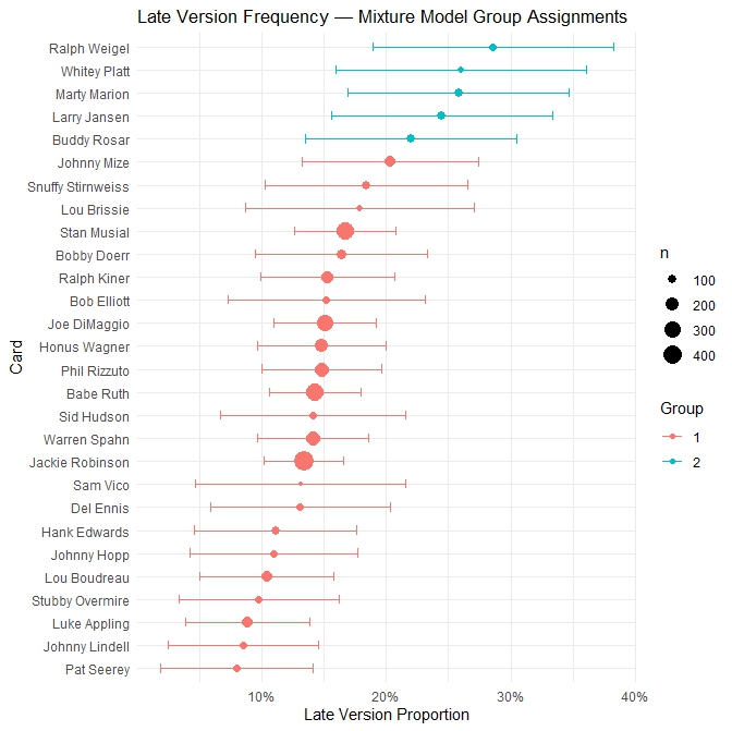
Step 11: Graph Results
A nice color-coded forest plot can now be generated.
df$ci_half <- 1.96 * sqrt(df$prop_b * (1 - df$prop_b) / df$n)

ggplot(df, aes(x = reorder(card_name, prop_b),
               y = prop_b,
               colour = factor(group))) +
  geom_point(aes(size = n)) +
  geom_errorbar(aes(ymin = prop_b - ci_half,
                    ymax = prop_b + ci_half),
                width = 0.4) +
  coord_flip() +
  scale_y_continuous(labels = scales::percent_format()) +
  labs(title  = "Late Version Frequency — Mixture Model Group Assignments",
       x      = "Card",
       y      = "Late Version Proportion",
       colour = "Group",
       size   = "n") +
  theme_minimal(base_size = 11)