It’s been a while since I publishing something, hasn’t it? I’ve been busy treasure hunting deep in the ’49 Leaf checklist.
Finding a short print from this set is always exciting, effectively combining my love of vintage cardboard with the extreme scarcity of the refractors I also chase. In fact, the second series names appear to exist on an individual basis in quantities not far removed from any given name in the ’93 Finest Refractor checklist. I have a half dozen of the Leaf SPs, and it is always a free-for-all when I need to battle other collectors to add one to this tally. I can only imagine what it would be like if Jackie Robinson or Joe DiMaggio had been in the short-printed second series rather than the first series.
As it turns out, Robinson, DiMaggio, and other massive names like Ruth and Musial have variations that are approximately SIX TIMES RARER than the cards in most collector’s collections. The crazy part? Nobody is looking for them. Nobody is advertising them. Nobody is paying a premium price. This sounds like an opportunity, one that can be acted upon at this very moment.
Brian Kappel’s Re: Leaf sent me down this path of research. He highlighted variations for the majority of the names appearing in the first series, variations resulting from a conscious decision to make these already colorful cards even brighter. After becoming convinced of the existence of these cards, the next logical line of inquiry was to ask about the relative scarcity of the two versions. Indeed, I am not the first to ask. Multiple interviewers have either asked Kappel about his thoughts on the matter or made their own projections. Most agreed that the “late” version, cards with brighter colored hats and additional border elements, were harder to find, but the numbers tossed around lacked a grounding in empirical data. These discussions were on the right track, but stopped before reaching the steps necessary to draw usable conclusions.
Could a more nuanced analysis of the data reveal a realistic estimate of the rarity of 1949 Leaf baseball cards?
What 1949 Leaf Variations Am I Talking About?
Let’s start this treasure hunt by defining the terms of engagement. I am looking for the relative populations of true variations that have yet to be formally recognized by hobby databases and price guides. Specifically, I am looking at a series of variations resulting from a decision at Leaf to mask off highly specific areas of black ink and simultaneously extend areas of high contrast color blocks along card borders. This is not a discussion of print defects or color differences resulting from the presses running low on ink.
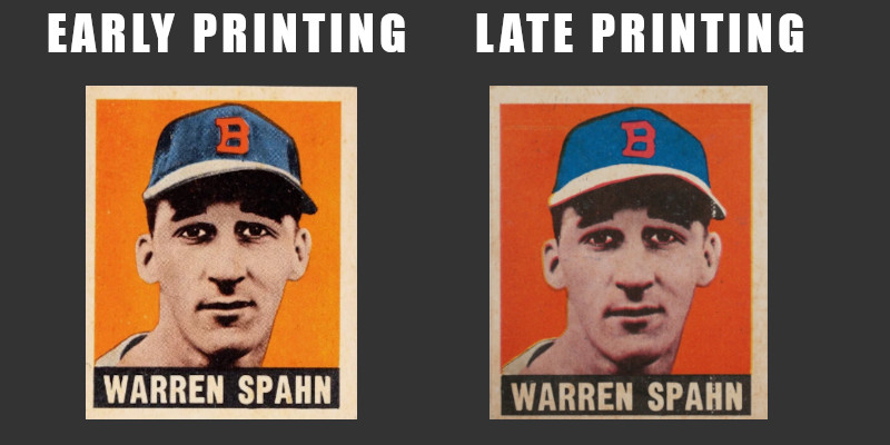
As an example, look at the Warren Spahn cards below. The one on the left represents the initial design of the card. It features a distinctly textured hat which was created by printing a semi-transparent layer of black ink on top of a solid blue background added earlier in the production process. The example on the left is the late printing variation, in which the black ink was intentionally masked off from the hat area. All other areas of black ink remain fully intact and adequately inked. The difference between these two cards is readily apparent when viewed side by side.
The same kind of hat color variation can be observed in the Johnny Mize card. As with Spahn, all black ink on the top of his ballcap has been masked off, resulting in a vibrant hat devoid of textural detail.
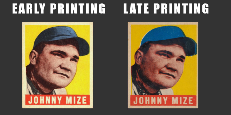
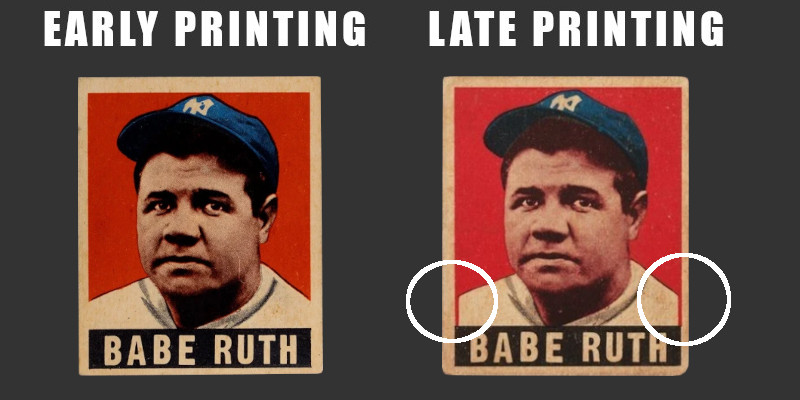
Variations between early and late printings are not solely limited to player hats. In addition to the removal of all detail from Mize’s hat, Leaf’s art department introduced a high contrast sliver of the colorful background to the space between the card border and the player jersey. Many of the modified names in the checklist contain a combination of changes to both hats and light colored border regions. Other cards, such as that of Babe Ruth, leave the hat alone and only feature the addition of the high contrast border lines.
These are generally minor changes, but they are intentional, repeated, and readily identifiable when one is looking for them. Leaf stopped the presses, edited their printing plates to improve the visual impact of the cards, and resumed shipments. The logical next step for any collector coming across this information is to ask if one version is rarer than the other.
Finding Data
So how should the problem of determining relative scarcity by approached? Leaf’s factory records seem lost to history, if any notes of this change were even committed to paper in the first place. Crowdsourcing a census is problematic, likely to yield only a small sample size that would be heavily influenced by the kind of collectors who go out of their way to collect obscure variations. I needed a sample from an agnostic source, and as Kappel learned firsthand, nobody cares less about these variations than PSA.
I started out by obtaining every single image from publicly reported sales of PSA graded Leaf cards, ultimately grabbing 3,471 images of unique serial numbers covering 28 different names in the checklist. This represents 19.7% of all PSA graded examples of these cards, a number that should provide a fairly robust sample. Why 28 cards instead of the 30+ Kappel identifies as having variations in his book? That is the number of cards that I could accurately identify which variation I was looking at in pictures. Why make this my sample set? The rationale was underpinned by four distinct pillars.
Pillar One: No Financial Incentive
There is zero observed pricing premium seen between any of the variations. It costs money to have cards slabbed, but that is somewhat irrelevant when it comes to the high dollar names like Jackie Robinson or Babe Ruth. Those cards are getting slabbed anytime someone wants to maximize their return when they market a card, resulting in slabbing rates that are not influenced by which variation a card happens to be. Grading costs, however, represent a much higher percentage of a card’s value for common players. If one variation carried a scarcity premium over another there would be a distinct incentive to grade the rare version over the common one, distorting the observed population. With no premium seeming to exist in published sales records, even the smaller population of common names should reflect a random sampling of the overall population.
A premium might eventually arise in pricing if long term “forever home” collectors were grabbing rare versions and systematically keeping them off the market in their forever collections. I found no evidence of an emerging premium so it stands to reason that a sample taken from two decades of grading reflects the general population of these cards “in the wild.”
Pillar Two: Nobody Cares
None of the major price guides, third party grading services, or hobby databases bother to break out separate listings for any of these variations. PSA does not differentiate between these variations on their labels. Their set registry considers a master set complete at 101 cards (98 base cards plus the 3 “official” variations recognized by the broader hobby). Even the completionists are ignoring these cards. This results in little to no incentive to seek out and slab whichever version is rarer on a “just because I want one of everything” basis. A search of active eBay listings shows almost zero awareness in listing titles of variations (just one active listing out of hundreds has any sort of mention of hat or border color).
Pillar Three: Serial Numbers
Every PSA slab has a unique serial number which I dutifully recorded. This was extraordinarily helpful in this project, as it allowed duplicate sales to be removed from the sample set. Each serial number is therefore represented exactly once in my data, regardless of how many times a particular card was relisted for sale across platforms or flipped between short term owners. This is a clean data set.
Pillar Four: Sampling a Different Source
Observing one out of every five Leaf cards ever graded by PSA seems like a pretty good sample to draw from, but it did leave some questions. Would the low number of observations of commons, some with as few as 48 appearances in the graded sample, be sufficient to draw conclusions? Does the PSA graded cohort actually mirror the unslabbed ’49 Leaf population in terms of observed variations?
To address these concerns, I sought to augment this information with more than 500 additional observations outside of the PSA ecosystem. I went to eBay and, looking only at active listings to avoid duplicating data, took a census of all non-PSA slabbed cards in my study. Sellers will not be advertising the same specific card across multiple active listings, making otherwise indistinguishable raw cards good for use as distinct data points. Potentially fraudulent listings were excluded, which were defined as any raw example of cards typically valued at above $1,000 (there are multiple Jackie Robinson and Babe Ruth “Etsy-specials” out there). I included graded cards from non-PSA grading services such as SGC and Beckett as well, further swelling the ranks of legit observations. This resulted in the following breakdown:
| PSA | Non-PSA | |
|---|---|---|
| Total Observations (n) | 3,471 | 510 |
| Early Printing Observations | 2,954 | 417 |
| % Early Printing | 85.1% | 81.8% |
| Late Printing Observations | 517 | 93 |
| % Late Printing | 14.9% | 18.2% |
| 95% Confidence | ±1.2% | ±3.4% |
| Confidence Interval | 13.7% – 16.1% | 14.8% – 21.6% |
The resulting ratio of early to late printing variations was fairly close between both sample sets, with the PSA cohort average (13.7% – 16.1%) overlapping with the confidence interval predicted by the non-PSA sample (14.8%-21.6%). As will be seen later, the overwhelming number of commons in the non-PSA sample might have even skewed the numbers further apart than they actually are. Still, the samples were looking pretty good and I now had almost 4,000 unique cards from which to draw conclusions.
What the Data Reveal About Relative Scarcity of Leaf Variations
Let’s start off with the big reveal: The late printing cards, the ones with supersaturated hats and high contrast borders, are demonstrably harder to find than the early printing versions. Late printing variations were found in 15.3% of the sample set, making them approximately 5.5x more scarce. That is a significant step up in rarity.
On top of this, the sample size produces a 95% confidence interval of ±1.2%, indicating high confidence in this result amid a very large sample set. Cutting that confidence interval in half would require another 11,943 observations, which is essentially a manual review of every single example of these ’49 Leaf card ever assessed by PSA. The sample we are working with shows we are not at the mercy of a handful of cards randomly skewing the data.
| CARD | COMPOSITE SAMPLE SIZE | % PSA TOTAL POP SAMPLED | % EARLY VERSION | % LATE VERSION | 95% CONFIDENCE INTERVAL |
|---|---|---|---|---|---|
| Jackie Robinson | 441 | 21.7% | 86.6% | 13.4% | ±3.2% |
| Babe Ruth | 343 | 19.6% | 85.7% | 14.3% | ±3.8% |
| Stan Musial | 323 | 22.0% | 83.3% | 16.7% | ±4.2% |
| Joe DiMaggio | 292 | 18.1% | 84.9% | 15.1% | ±4.1% |
| Warren Spahn | 234 | 17.7% | 85.9% | 14.1% | ±4.5% |
| Phil Rizzuto | 209 | 19.6% | 85.2% | 14.8% | ±5.0% |
| Honus Wagner | 182 | 18.7% | 85.2% | 14.8% | ±5.3% |
| Ralph Kiner | 170 | 19.8% | 84.7% | 15.3% | ±5.7% |
| Lou Boudreau | 125 | 20.0% | 89.6% | 10.4% | ±5.8% |
| Luke Appling | 124 | 18.5% | 91.1% | 8.9% | ±5.3% |
| Johnny Mize | 123 | 19.2% | 79.7% | 20.3% | ±7.7% |
| Bobby Doerr | 110 | 18.5% | 83.6% | 16.4% | ±7.3% |
| Marty Marion | 93 | 19.8% | 74.2% | 25.8% | ±10.3% |
| Buddy Rosar | 91 | 19.5% | 78.0% | 22.0% | ±10.2% |
| Larry Jansen | 90 | 16.3% | 75.6% | 24.4% | ±11.3% |
| Hank Edwards | 90 | 19.2% | 88.9% | 11.1% | ±7.6% |
| Snuffy Stirnweiss | 87 | 19.0% | 81.6% | 18.4% | ±9.6% |
| Sid Hudson | 85 | 22.3% | 85.9% | 14.1% | ±8.6% |
| Ralph Weigel | 84 | 18.4% | 71.4% | 28.6% | ±12.0% |
| Del Ennis | 84 | 18.6% | 86.9% | 13.1% | ±8.0% |
| Stubby Overmire | 82 | 15.7% | 90.2% | 9.8% | ±8.3% |
| Johnny Hopp | 82 | 16.4% | 89.0% | 11.0% | ±8.3% |
| Johnny Lindell | 82 | 17.5% | 91.5% | 8.5% | ±7.0% |
| Bob Elliot | 79 | 19.7% | 84.8% | 15.2% | ±8.3% |
| Pat Seerey | 75 | 20.2% | 92.0% | 8.0% | ±7.0% |
| Whitey Platt | 73 | 20.6% | 74.0% | 26.0% | ±12.0% |
| Lou Brissie | 67 | 18.4% | 82.1% | 17.9% | ±10.6% |
| Sam Vico | 61 | 15.4% | 86.9% | 13.1% | ±9.5% |
| Group Level Total | 3,981 | 19.7% | 84.7% | 15.3% | ±1.2% |
So far, so good. We can definitively declare the late version to not just be harder to find than the earlier version; we find the scarcity of these cards to be multiples of the early “dark hat” versions. The next question to answer is whether or not that 15.3% late printing ratio applies to all cards.
All of these cards come from Series One of the ’49 Leaf checklist, and all originated from a 7×7 grid on the same 49-card master printing sheet. A single, solitary changeover from the early version of the printing plates to the reworked later version at a discrete point in time would produce equal ratios of late variations for every affected name in the checklist. That makes sense, right? That is why it was my working theory when I saw so many of the high population cards clustering so tightly around 15.3%.
However, if you have been studying the above table, something stands out as being incongruous with the idea of a one time modification of the printing plates.
We Have a Problem…
The 8 cards with the highest number of observations all cluster tightly around 15%, as would be expected in a population undergoing a one time printing plate adjustment. However, things start getting weird beyond that point. Luke Appling, with well over 100 observations, and names like Johnny Lindell and Pat Seerey have late printing frequencies of around 10%. Meanwhile, Marty Marion, Larry Jansen, and Ralph Weigel appear to have late variations show up in nearly 25% of all observations. Are these wildly varying Late Version frequencies just noise from having a lower quantity of observations? Do I just need to find more Pat Seerey cards?
We can do a quick visual check of the data to provide some insight. Below appear selected names of interest.
| Name | n Observations | Early Printing | Late Printing | Confidence Interval |
|---|---|---|---|---|
| Luke Appling | 124 | 91.1% | 8.9% | ±5.3% |
| Pat Seerey | 75 | 92.0% | 8.0% | ±7.0% |
| Johnny Lindell | 82 | 91.5% | 8.5% | ±7.0% |
| Ralph Weigel | 84 | 71.4% | 28.6% | ±12.0% |
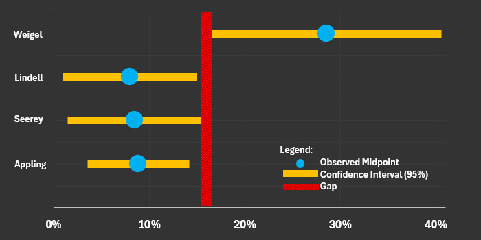
In the plot above, we see the estimated late printing frequencies with a wide gulf for Appling (8.9%), Seerey (8.0%), Lindell (8.5%), and Weigel (28.6%). Obviously, the true frequency of late printings can be different than these precise sounding numbers. To show how far these frequencies can drift from these observations, the illustration also includes confidence interval bands as blue bars around these estimates.
The intervals are drawn to 95% confidence, implying a 95% probability that the true frequencies of the populations reside somewhere inside those ranges. If these variations were all created at once from a one-time change to the master sheet, we should see these ranges overlapping. The smaller number of observations for the Weigel card and its higher frequency of late version observations warrant a much wider confidence interval than Appling. The same confidence still holds for Weigel, it just covers a double digit range of possibilities, swinging 12% in either direction. The 28.6% late frequency is just my best estimate, based on the cards observed, but the true population could easily be anywhere from 16.6% to 40.6%.
Graphing the distribution of these outliers with their confidence intervals reveals something. When we graph the distribution of these names we find a massive gap that even a double digit confidence interval cannot overcome. The odds of random noise in the data or a small sample size being the root cause of this gap are almost zero. The 14.2% upper bound of Appling sits entirely below Weigel’s lower bound (16.6%). Their confidence intervals do not overlap at all. The same is true for Seerey or Lindell vs. Weigel, as well as several other comparative combinations in the checklist. This means there is no single proportion that falls within the confidence interval of all 28 cards simultaneously, a key test for homogeneity, even after accounting for the differences in number of observations.
While many individual pairs of confidence intervals do broadly overlap, the constrains from the intervals at the high and low end are mutually exclusive. Because these gaps exist between cards like Appling and Weigel, we can effectively rule out the idea that all of these variations exist in the same ratios – the condition that would result from a one time modification of the production machinery. Leaf apparently introduced these changes at different points in time.
Testing For Multiple Modifications
If Leaf stopped multiple times along the way to adjust the printing plates, there would be different ratios (and by extension different levels of relative scarcity) for early and late variations of specific cards. But I have one giant pile of data. What tool could be used to tease out the existence of multiple bell curves hiding inside my sample?
The answer is a mixture model. These models assume observed data comes from a combination of multiple underlying probability distributions and can identify the component distributions and their relative weights. In theory, this could not only lead to the discovery of how many batches of variations Leaf made, but to the identity of the cards that fall within each group as well. For those that are interested, the full methodology, source file, and R code are outlined separately. These models can quickly get complicated outside of a spreadsheet or computer file, so I am only reporting the results of its output on this page.
Here is what I found:
Based on the model output, Leaf appears to have created two distinct batches of variations. The 3.20 point improvement in BIC (one of the metrics for scoring this model) was a modest positive in favor of two batches over one, while a simultaneous improvement in AIC (another scoring metric) was a more persuasive 5.87. Importantly, both point in the same direction and to the same conclusion. Coupled with the gap between potential confidence intervals seen in the initial independent analysis, it quickly becomes apparent that the late printing variations spring out of two distinct series of modifications to the master printing plates. The model produced a plot showing the breakdown within these two groups.
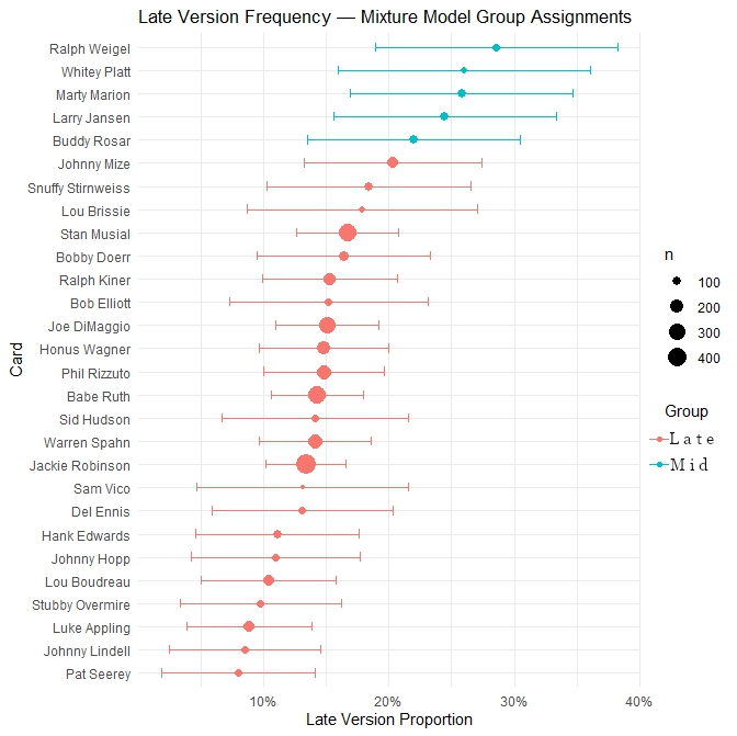
The “Middle/Late Printing” variations (depicted in blue) represents 5 cards that were likely adjusted at an earlier point in the production cycle and thus have a greater proportion in circulation. They are much easier to find, but still clock in as being about three times more scarce than the early printing variations with dark hats.
The “Very Late Printing” group, comprising 23 of the studied names and depicted in red, consists of the bulk of the affected cards. These brighter hat/extended border cards appear to be almost six times harder to find than the more common dark hat/early printing variations.
| Description | Middle/Late Printing | Very Late Printing |
|---|---|---|
| Players Depicted (out of 28 studied) | 5 | 23 |
| Timing of Plate Adjustment | Between Early (Dark Hats) and Very Late Printing | After Middle Group |
| Mean Frequency of Early Printing Variations | 74.710% | 85.045% |
| Mean Frequency of Late Printing Variations | 25.290% | 14.955% |
| Confidence Interval (95%) | ±4.104% | ±1.208% |
| Observations (n) | 431 | 3,550 |
| Implied Rarity Relative to Early Printing Variation | 2.95x | 5.69x |
Two cards are flagged by the model as being rather ambiguous as to which group they truly belong to. While additional observations might swing them in one direction or the other, Johnny Mize barely squeezes into the Very Late Printing Group while Buddy Rosar is slightly more likely to be part of the more common Mid/Late Printing.
A Theory for ‘Why?’
So why would there be changes made to the printing plates on multiple, completely separate production runs? There are many plausible answers to this question, ranging from the uneven wear necessitating early replacement of some plates to a temperamental artist being employed to print tiny pictures of baseball players in a candy company factory. Out of the countless possibilities, my favorite theory of what created the switch is a simple A/B test of consumer preferences. Here’s how such a scenario could have played out.
The timing of modifications of these cards at multiple points in the production timeline potentially makes sense when you step back and think about the operational need of Leaf’s production floor and the printing method employed. The cards were printed on a four color industrial offset press on the same cardstock used to package the company’s candy displays. As Kappel hypothesizes in his book, the cards were likely printed by a swing shift when the printing equipment would otherwise be idle, with Leaf essentially making cards using the excess capacity of the manpower and equipment used to print their packaging materials. The heavy plates would need to be bolted into the machine, large rubber cylinders would need to be inked and inserted into their correct positions, and cardstock would need to be fed into the apparatus, a series of events that took four separate passes to complete with ample drying time between each one. There simply wasn’t a surplus of downtime in which to make time consuming changes without disrupting production for an extended time.
At some point a decision was made to adjust the printing plates to make the cards more visually appealing. It would make sense to conduct a test before engaging in the time consuming process of adjusting printing plates for the entire sheet. The late versions with the highest observed frequency would be the prime candidates for testing, as they apparently exist in larger numbers than the others. 5 of the 28 names in this study have an average late version frequency of 25% and appear to be good candidates for this “test” group. This list is comprised of the less popular (i.e. expendable) names in the checklist (Platt, Weigel, Rosar, Jansen, and Marion), making them prime candidates for experimentation. Kids would be upset if Babe Ruth’s card didn’t turn out well. Whitey Platt? Not so much.
Could the placement of these cards on the master sheet also have something to do with testing ink flow to various regions of the newly modified master sheet? A case can be made for this if one squints really hard at the layout, but this may be taking things too far.
With the test apparently successful, the next round of adjustments hit almost all the big names in the checklist: DiMaggio; Musial; Spahn; Rizzuto; Wagner; Jackie; and, of course, the Bambino.
What Does This Imply For Collectors?
Does having multiple variations to chase in an iconic vintage set affect the way we collect? Not always. Few seem to care about discerning between the red and black back cards in the 1952 Topps issue. The hobby largely treats the ’52 varieties as interchangeable, assigning no pricing premium despite the black back version being approximately one third rarer than the red backs (the population is ~40% black versus ~60% red back). A handful of master set builders care deeply about this, but there are simply more cards in circulation than there are collectors who seek this level of granularity.
Am I obsessing over ’49 Leaf variations that are actually buried in the same level of indifference? I don’t think so. Aside from the much smaller print run of Leaf cards compared to Topps, there is a precedent for how collectors react to these exact early/late printing variations.
Here I turn to looking at the sets Kent Peterson card, the sole “early printing/late printing” variation widely recognized within the hobby. I had initially dismissed it from my population study because collector interest polluted the incentives around the card. The premium ascribed to the “red hat” (i.e. late printing) variation shows collectors do not just care about the card, they exhibit a material preference for it, pushing up its value and inducing a steady flow of red hat versions towards PSA compared to the more common variety. I suspect this card actually exists in quantities equal to one of the batches of variations observed in my study and would expect a similar demand and pricing dynamic could potentially emerge for the other later variations should their existence become widely recognized among collectors.
The Treasure Map
I started off deliberately phrasing this study as a treasure hunt. The underlying numbers and exhibited collector behavior towards the Peterson card are uniformly pointing towards a likely outcome: Collectors will eventually ascribe a scarcity premium to most, if not all, of the late printing variations. The master checklist just expanded by dozens of cards, collectors haven’t realized it yet, and the odds are most of these collections only have the more common variety in hand. How will they react?
For this I again look to the Peterson card for a directional guide and a rough approximation of what the future state of the market for these cards could look like. The red hat (late printing) Peterson typically sells for a 2.6x-3.1x premium compared to the black hat variety. Can you imagine the bifurcated market that could potentially develop for the biggest names in the set if they too reflected a similar premium? It would fundamentally alter the way collectors approach a set whose mythology has already shifted multiple times over nearly 80 years.
Here is how I am directly applying this to my collection. I would like to one day complete this set. As things currently stand, I can pick up the scarce varieties of these cards for the same outlay as would be required to acquire the common early printing variations. I can purposely organize my shopping list around hard to find cards that nobody else seems to be seeking out, systematically picking up structurally scarcer versions. If a premium does develop, I can trade the rare varieties I have locked away for higher grade examples of common early printings or, more likely, use the proceeds from selling rare cards to fund equally graded early print examples and apply the surplus funds to finance the scary expensive names that currently elude me. How great would it be to pick up a handful of Hall of Famers and later exchange them for the exact same names plus a Bob Feller or Hal Newhouser short print? This is the treasure hunt scenario that currently exists and is one that I have been actively pursuing.
While this scenario could easily just be wishful thinking, it is at least asymmetric wishful thinking. If no scarcity premium develops over time I still have awesome cards that I know are much, much more difficult to find than the typical ’49 Leaf cardboard. Sure, this rarity might be based on observing minor, almost invisible echoes of a postwar printing press swing shift, but that is the kind of thing I love to dig into. The cards have a hidden story. They are exactly the sort of cards I want in my collection and I would be happy to be “stranded” with the late printing variations as the cornerstone of my set.